4f Optical Correlator#
This notebook is the entry point for the 4f family in the example set. It introduces a coherent 4f optical correlator that uses a matched filter to locate copies of a target pattern inside a larger scene.
Code is synced from scripts/4f_correlator.py.
Assumes you know#
basic coherent propagation and complex fields,
what a Fourier transform does, and
how intensity is measured from a complex field.
New ideas in this notebook#
why the optical path
prop(f) -> lens(f) -> prop(f)implements a Fourier transform,how to choose the sampling-matched focal length so the Fourier-plane grid lines up with the simulation grid,
why a matched filter produces cross-correlation peaks, and
what paraxial assumption makes this construction valid.
Where to go next#
If this notebook makes sense, continue to 4f_edge_optimization.ipynb. That notebook reuses the same 4f geometry and focuses only on the new ingredient: learning a phase-only Fourier-plane filter for edge detection.
Outline#
Imports for optics components and numerics.
Paths and Parameters for saved artifacts.
Concept and helper functions with physics background (Fourier-transforming lens, sampling-matched focal length, matched filter, paraxial validity).
Setup of the 4f correlator optical system.
Evaluation and comparison with direct FFT cross-correlation.
Plot Results for visual inspection.
0 Imports#
We import fouriax optics components together with NumPy/Matplotlib utilities for the
discrete 4f simulation and the final comparison plots.
from __future__ import annotations

from pathlib import Path

import jax.numpy as jnp
import matplotlib.pyplot as plt
import numpy as np

import fouriax as fx
%matplotlib inline

EXAMPLES_ROOT = Path.cwd() / "examples"
EXAMPLES_ARTIFACTS_DIR = EXAMPLES_ROOT / "artifacts"
1 Paths and Parameters#
This section fixes the wavelength, refractive index, grid sampling, and artifact path used for the baseline correlator experiment.
ARTIFACTS_DIR = Path(str(EXAMPLES_ARTIFACTS_DIR))
PLOT_PATH = ARTIFACTS_DIR / "4f_correlator.png"

WAVELENGTH_UM = 0.532
N_MEDIUM = 1.0
GRID_N = 128
GRID_DX_UM = 2.0
PLOT = True
2 Concept and Helper Functions#
This is the reusable theory section for the 4f notebooks. Later notebooks in this family should point back here for geometry and sampling, then explain only their new optical element or objective.
Fourier-transforming property of a lens#
A coherent field \(E_{\text{in}}(x)\) placed at the front focal plane of a thin lens of focal length \(f\) produces, at the back focal plane, the field
In words: the output is the spatial Fourier transform of the input, evaluated at spatial frequency \(f_x = x'/(\lambda f)\), up to a constant prefactor.
Crucially, the input must be at the front focal plane — a distance \(f\) before the lens — for this to hold without a residual quadratic-phase term. The complete path for one Fourier-transforming stage is therefore
Sampling-matched focal length#
We simulate on a discrete \(N \times N\) grid with pixel spacing \(\Delta x\). The highest spatial frequency the grid can represent is \(f_{x,\max} = 1/(2\Delta x)\) (the Nyquist frequency). At the Fourier plane, this frequency maps to position
For the Fourier-plane grid to have the same pixel spacing \(\Delta x\) and the same number of samples \(N\), we need
where \(n\) is the refractive index of the medium. This is the sampling-matched focal length. It guarantees a one-to-one mapping between the DFT frequency bins and the physical positions at the Fourier plane.
The matched filter#
A 4f system places two Fourier-transforming stages back to back with a filter mask at the shared Fourier plane:
Without the filter (\(H = 1\)), the two Fourier transforms compose to give a spatially inverted copy of the input — a trivial imaging system.
With a matched filter
the output field becomes (up to constants)
which is exactly the cross-correlation of the scene \(S\) with the target \(T\) (by the correlation theorem). The output intensity \(|E_{\text{out}}|^2\) will show bright peaks wherever the target pattern appears in the scene.
Paraxial validity constraint#
The thin-lens Fourier-transform relationship relies on the paraxial approximation: rays make small angles with the optical axis. The worst case is a ray from the edge of the grid (\(r_{\max} = N\Delta x / 2\)) to the lens centre, subtending an angle \(\theta \approx r_{\max}/f\).
Using the sampling-matched focal length,
which depends only on \(\lambda\) and \(\Delta x\) — not on \(N\). We need this ratio \(\ll 1\) for the paraxial approximation to hold. Choosing \(\Delta x \gg \lambda/(2n)\) ensures this.
def _raw_correlate(scene: jnp.ndarray, target: jnp.ndarray) -> jnp.ndarray:
    """Ground-truth cross-correlation intensity via direct FFT."""
    f_scene = jnp.fft.fftn(jnp.fft.ifftshift(scene), axes=(-2, -1))
    f_target = jnp.fft.fftn(jnp.fft.ifftshift(target), axes=(-2, -1))
    corr = jnp.fft.ifftn(f_scene * jnp.conj(f_target), axes=(-2, -1))
    return jnp.abs(jnp.fft.fftshift(corr)) ** 2


def _sampling_matched_focal_length(grid: fx.Grid) -> float:
    """f = n·N·dx² / λ"""
    return N_MEDIUM * grid.nx * grid.dx_um**2 / WAVELENGTH_UM


def _matched_filter(target: jnp.ndarray) -> tuple[jnp.ndarray, jnp.ndarray]:
    """Fourier-plane matched filter: (amplitude, phase_rad).

    Built in the centred (fftshift) convention to match the physical
    Fourier plane, where DC sits at the optical axis.
    """
    ft = jnp.fft.fftshift(
        jnp.fft.fftn(jnp.fft.ifftshift(target), axes=(-2, -1)),
        axes=(-2, -1),
    )
    amplitude = jnp.abs(ft) / jnp.max(jnp.abs(ft))
    phase_rad = -jnp.angle(ft)
    return amplitude, phase_rad


def _paraxial_validity_constraint_fom() -> float:
    """Dimensionless paraxial figure-of-merit (r_max / f)^2 for this grid pitch."""
    return (WAVELENGTH_UM / (2 * N_MEDIUM * GRID_DX_UM)) ** 2


def _make_rect(grid: fx.Grid, cx_f: float, cy_f: float, w_f: float, h_f: float) -> jnp.ndarray:
    """Binary rectangle; positions/sizes are fractions of grid half-extent."""
    half = grid.nx * grid.dx_um / 2.0
    x, y = grid.spatial_grid()
    return (
        (jnp.abs(x - cx_f * half) <= w_f * half) & (jnp.abs(y - cy_f * half) <= h_f * half)
    ).astype(jnp.float32)


def _build_scene(grid: fx.Grid) -> jnp.ndarray:
    """Three copies of the target square plus a distractor rectangle."""
    hw = 0.10
    scene = jnp.zeros(grid.shape, dtype=jnp.float32)
    for cx, cy in [(-0.35, -0.25), (0.20, 0.38), (0.40, -0.20)]:
        scene = scene + _make_rect(grid, cx, cy, hw, hw)
    scene = scene + 0.5 * _make_rect(grid, -0.18, 0.20, 0.18, 0.05)
    return jnp.clip(scene, 0.0, 1.0)


def _build_target(grid: fx.Grid) -> jnp.ndarray:
    """Centred target square (same size as copies in the scene)."""
    return _make_rect(grid, 0.0, 0.0, 0.10, 0.10)
3 Setup#
We now instantiate the base 4f system described above. The same lens-propagation geometry will be reused by later notebooks in this family.
The optical system uses ASMPropagator (Angular Spectrum Method) with the
sampling planner disabled so that the grid spacing stays exactly matched
to the focal length.
The output is spatially inverted because two successive Fourier transforms flip the image. We flip it back for comparison with the ground truth.
grid = fx.Grid.from_extent(nx=GRID_N, ny=GRID_N, dx_um=GRID_DX_UM, dy_um=GRID_DX_UM)
spectrum = fx.Spectrum.from_scalar(WAVELENGTH_UM)
f_um = _sampling_matched_focal_length(grid)
print(f"f = {f_um:.1f} µm  |  (r_max/f)² = {_paraxial_validity_constraint_fom():.4f}")

scene = _build_scene(grid)
target = _build_target(grid)
field_in = fx.Field.plane_wave(grid=grid, spectrum=spectrum).apply_amplitude(scene[None, :, :])

amp, phase = _matched_filter(target)

prop = fx.plan_propagation(
    mode="auto",
    grid=grid,
    spectrum=spectrum,
    distance_um=f_um,
)
lens = fx.ThinLens(focal_length_um=f_um)

correlator = fx.OpticalModule(
    layers=(
        prop,
        lens,
        prop,
        fx.ComplexMask(amplitude_map=amp, phase_map_rad=phase),
        prop,
        lens,
        prop,
    ),
    sensor=fx.DetectorArray(detector_grid=grid),
)
f = 962.4 µm | (r_max/f)² = 0.0177
4 Evaluation#
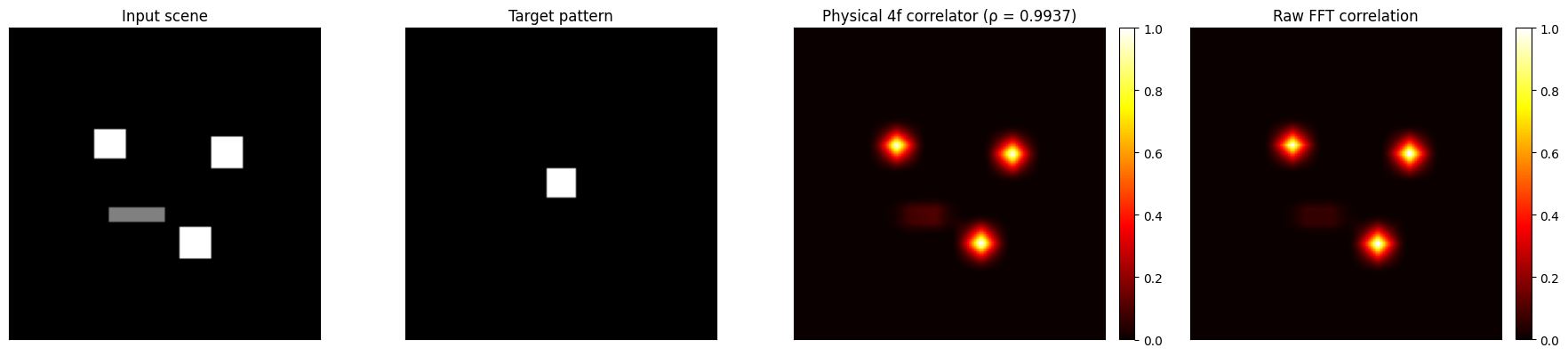
We compare the simulated 4f output against direct FFT-based cross-correlation on the same scene. High agreement confirms that the optical construction reproduces the expected matched-filter computation.
output_4f = np.asarray(correlator.measure(field_in))
output_raw = np.asarray(_raw_correlate(scene, target))

output_4f = output_4f[::-1, ::-1]
norm = lambda x: x / np.max(x) if np.max(x) > 0 else x  # noqa: E731
out_4f_n, out_raw_n = norm(output_4f), norm(output_raw)
cc = float(np.corrcoef(out_4f_n.ravel(), out_raw_n.ravel())[0, 1])
print(f"Correlation with ground truth: {cc:.4f}")
Correlation with ground truth: 0.9937
5 Plot Results#
The main visual check is that bright peaks appear at the target locations and that the optical correlator matches the direct numerical reference.
Next notebook#
After this, 4f_edge_optimization.ipynb keeps the same 4f layout but replaces the fixed matched filter with a trainable phase-only Fourier-plane filter.
if PLOT:
    fig, axes = plt.subplots(1, 4, figsize=(18, 4))
    axes[0].imshow(np.asarray(scene), cmap="gray")
    axes[0].set_title("Input scene")
    axes[1].imshow(np.asarray(target), cmap="gray")
    axes[1].set_title("Target pattern")

    for ax, img, title in zip(
        axes[2:],
        [out_4f_n, out_raw_n],
        [f"Physical 4f correlator (ρ = {cc:.4f})", "Raw FFT correlation"],
        strict=True,
    ):
        im = ax.imshow(img, cmap="hot")
        ax.set_title(title)
        fig.colorbar(im, ax=ax, fraction=0.046, pad=0.04)

    for ax in axes:
        ax.set_xticks([])
        ax.set_yticks([])
    fig.tight_layout()

    ARTIFACTS_DIR.mkdir(parents=True, exist_ok=True)
    fig.savefig(PLOT_PATH, dpi=150)
    plt.show()
    print(f"saved: {PLOT_PATH}")
saved: /Users/liam/metasurface/fouriax/examples/artifacts/4f_correlator.png