Incoherent Camera Imaging — PSF and OTF Modes#
This is a standalone advanced notebook. It models a shift-invariant incoherent imaging system
with IncoherentImager and compares two numerically equivalent implementations of image formation:
mode="psf", which performs convolution in the spatial domain.mode="otf", which performs multiplication in the frequency domain.
Modeling assumptions#
illumination is incoherent, so object intensities add linearly through the PSF,
the imaging system is treated as shift-invariant over the simulated field of view, and
both modes are derived from the same lens, propagator, and PSF normalization choice.
The goal is not to optimize a design, but to verify that the two incoherent-imaging formulations agree for the same optical system.
0 Imports#
The notebook uses NumPy and Matplotlib for diagnostics and the fouriax imaging stack for the lens,
Rayleigh-Sommerfeld propagation, incoherent image formation, and detector-array readout.
from __future__ import annotations

from pathlib import Path

import jax.numpy as jnp
import matplotlib.pyplot as plt
import numpy as np

import fouriax as fx
%matplotlib inline

EXAMPLES_ROOT = Path.cwd() / "examples"
EXAMPLES_ARTIFACTS_DIR = EXAMPLES_ROOT / "artifacts"
1 Paths and Parameters#
The parameters set the scalar wavelength, grid sampling, focal length, aperture diameter, and sensor crop size. Together they determine the effective numerical aperture and the portion of the simulated image plane reported as the sensor region of interest.
ARTIFACTS_DIR = Path(str(EXAMPLES_ARTIFACTS_DIR))
PLOT_PATH = ARTIFACTS_DIR / "incoherent_camera.png"

WAVELENGTH_UM = 0.532
GRID_N = 192
GRID_DX_UM = 1.0
F1_UM = 2700.0
F2_UM = 1350.0
APERTURE_DIAMETER_UM = 90.0
SENSOR_SIZE_PX = 96
PLOT = True
PARAXIAL_MAX_ANGLE_RAD = 0.05
2 Helper Functions#
The helper functions define a synthetic object intensity with several spatial scales and a simple center crop used to emulate a finite sensor ROI. The object is deliberately varied enough to make PSF blur and parity checks visually obvious.
def _make_object_intensity(grid: fx.Grid) -> jnp.ndarray:
    x, y = grid.spatial_grid()
    r = jnp.sqrt(x * x + y * y)
    disk = (r <= 20.0).astype(jnp.float32)
    ring = ((r >= 32.0) & (r <= 40.0)).astype(jnp.float32)
    bars = (jnp.cos(2.0 * jnp.pi * x / 9.0) > 0.0).astype(jnp.float32)
    envelope = jnp.exp(-((r / 48.0) ** 2))
    return jnp.clip(0.05 + 0.45 * disk + 0.25 * ring + 0.25 * bars * envelope, 0.0, 1.0)


def _grid_extent_um(grid: fx.Grid) -> tuple[float, float, float, float]:
    half_width_um = 0.5 * grid.nx * grid.dx_um
    half_height_um = 0.5 * grid.ny * grid.dy_um
    return (-half_width_um, half_width_um, -half_height_um, half_height_um)


def _grid_extent_angle_mrad(grid: fx.Grid, distance_um: float) -> tuple[float, float, float, float]:
    half_width_mrad = 1e3 * (0.5 * grid.nx * grid.dx_um) / distance_um
    half_height_mrad = 1e3 * (0.5 * grid.ny * grid.dy_um) / distance_um
    return (-half_width_mrad, half_width_mrad, -half_height_mrad, half_height_mrad)


def _angle_pitch_mrad(grid: fx.Grid, distance_um: float) -> tuple[float, float]:
    return 1e3 * grid.dx_um / distance_um, 1e3 * grid.dy_um / distance_um
3 Setup#
We construct a thin lens plus a Rayleigh-Sommerfeld propagator, then instantiate two
IncoherentImager modules that differ only in implementation mode: one builds images from the PSF,
the other from the OTF.
For a shift-invariant incoherent system with object intensity \(o(x,y)\) and point-spread function \(h(x,y)\), the image intensity is
The optical transfer function is the Fourier transform of the PSF,
so the same image can be written in the frequency domain as
Because both modules share the same optics, any discrepancy between their outputs is numerical rather than conceptual.
# Keep the example same-shape while allowing smoke tests to shrink workload.
sensor_n = min(GRID_N, SENSOR_SIZE_PX)
sensor_grid = fx.Grid.from_extent(nx=sensor_n, ny=sensor_n, dx_um=GRID_DX_UM, dy_um=GRID_DX_UM)
spectrum = fx.Spectrum.from_scalar(WAVELENGTH_UM)
if F1_UM <= 0 or F2_UM <= 0:
    raise ValueError("f1_um and f2_um must be strictly positive")

object_distance_um = F1_UM
image_distance_um = F2_UM
focal_length_um = 1.0 / ((1.0 / object_distance_um) + (1.0 / image_distance_um))
magnification_abs = image_distance_um / object_distance_um

lens_na = APERTURE_DIAMETER_UM / (2.0 * image_distance_um)

lens = fx.ThinLens(
    focal_length_um=focal_length_um,
    aperture_diameter_um=APERTURE_DIAMETER_UM,
)
rs = fx.RSPropagator(
    use_sampling_planner=True,
    warn_on_regime_mismatch=False,
    refractive_index=1.0,
)

input_grid = fx.Grid.from_extent(
    nx=sensor_grid.nx,
    ny=sensor_grid.ny,
    dx_um=sensor_grid.dx_um / magnification_abs,
    dy_um=sensor_grid.dy_um / magnification_abs,
)

imager_psf = fx.IncoherentImager.for_finite_distance(
    optical_layer=lens,
    propagator=rs,
    input_distance_um=object_distance_um,
    output_distance_um=image_distance_um,
    normalize_psf=True,
    mode="psf",
)
imager_otf = fx.IncoherentImager.for_finite_distance(
    optical_layer=lens,
    propagator=rs,
    input_distance_um=object_distance_um,
    output_distance_um=image_distance_um,
    normalize_psf=True,
    mode="otf",
)
object_intensity = fx.Intensity(
    data=_make_object_intensity(input_grid)[None, :, :],
    grid=input_grid,
    spectrum=spectrum,
)
sensor_width_um = sensor_grid.nx * sensor_grid.dx_um
input_width_um = input_grid.nx * input_grid.dx_um
half_object_fov_deg = float(np.degrees(np.arctan((input_width_um * 0.5) / object_distance_um)))
object_fov_deg = 2.0 * half_object_fov_deg
input_dtheta_x_mrad, input_dtheta_y_mrad = _angle_pitch_mrad(input_grid, object_distance_um)
sensor_dtheta_x_mrad, sensor_dtheta_y_mrad = _angle_pitch_mrad(sensor_grid, image_distance_um)

detector_array = fx.DetectorArray(
    detector_grid=sensor_grid,
    qe_curve=1.0,
)
field_template = fx.Field.zeros(grid=input_grid, spectrum=spectrum)
4 Evaluation#
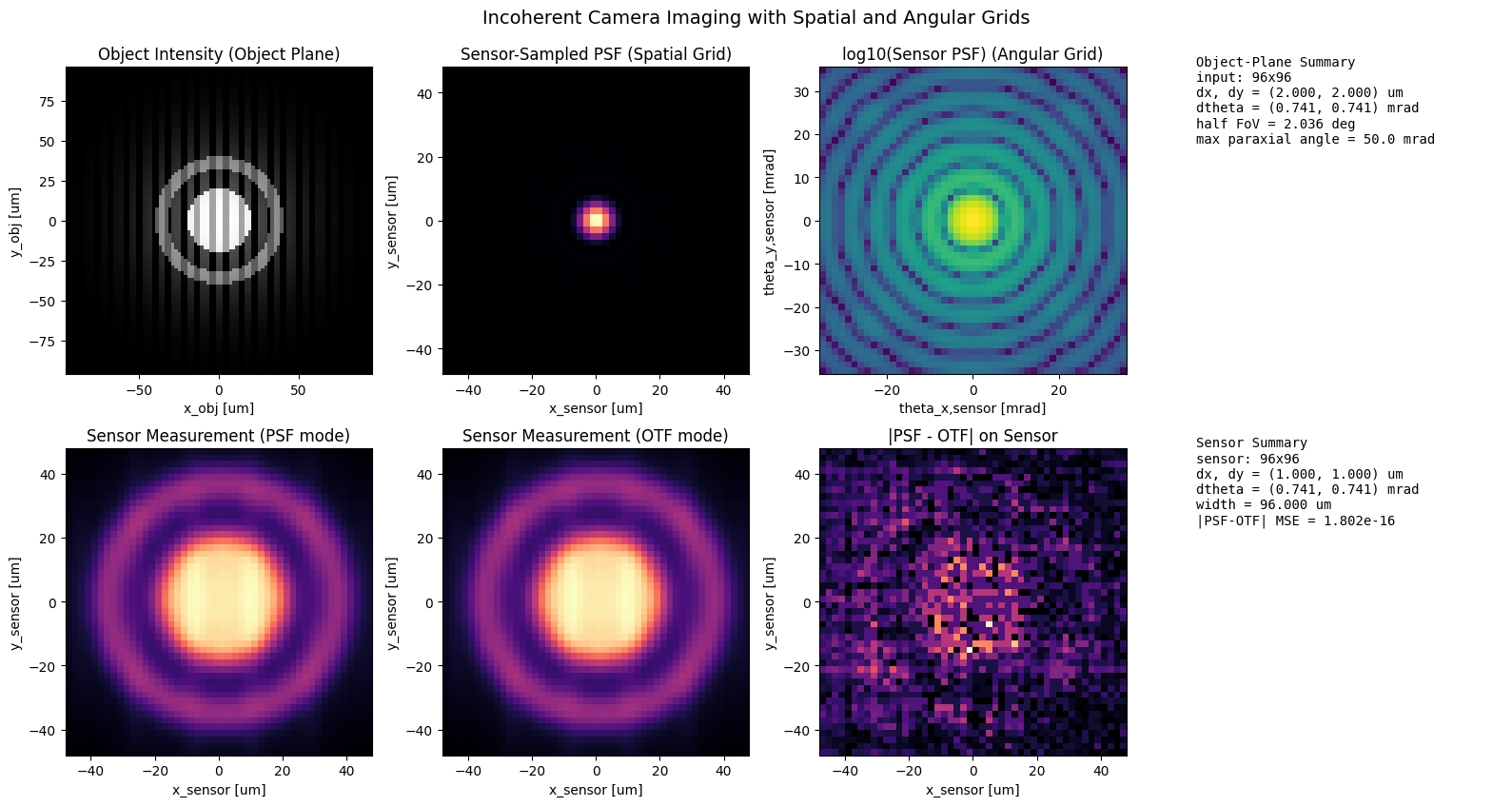
We measure the same incoherent object with both imaging modes, compare the full-frame outputs, and also compare a central sensor crop. The reported parity MSE values are the main quantitative check that PSF-mode and OTF-mode imaging agree for this example.
image_psf = np.asarray(detector_array.measure(imager_psf.forward(object_intensity)))
image_otf = np.asarray(detector_array.measure(imager_otf.forward(object_intensity)))

parity_mse_sensor = float(np.mean((image_psf - image_otf) ** 2))
print("=== Incoherent Camera Example ===")
print(f"f1_um={object_distance_um:.1f}")
print(f"f2_um={image_distance_um:.1f}")
print(f"derived_focal_length_um={focal_length_um:.1f}")
print(
    "thin_lens_residual="
    f"{(1.0 / focal_length_um) - (1.0 / object_distance_um) - (1.0 / image_distance_um):.3e}"
)
print(f"magnification_abs={magnification_abs:.3f}")
print(f"aperture_diameter_um={APERTURE_DIAMETER_UM:.1f}")
print(f"effective_na={lens_na:.4f}")
print(f"paraxial_max_angle_rad={PARAXIAL_MAX_ANGLE_RAD:.3f}")
print(f"input_grid_shape={input_grid.ny}x{input_grid.nx}, input_dx_um={input_grid.dx_um:.3f}")
print(
    f"input_dtheta_mrad=({input_dtheta_x_mrad:.3f}, {input_dtheta_y_mrad:.3f})"
)
print(
    f"sensor_grid_shape={sensor_grid.ny}x{sensor_grid.nx}, "
    f"sensor_dx_um={sensor_grid.dx_um:.3f}"
)
print(
    f"sensor_dtheta_mrad=({sensor_dtheta_x_mrad:.3f}, {sensor_dtheta_y_mrad:.3f})"
)
print(f"input_width_um={input_width_um:.3f}, sensor_width_um={sensor_width_um:.3f}")
print(f"half_object_fov_deg={half_object_fov_deg:.3f}, object_fov_deg={object_fov_deg:.3f}")
print(f"PSF/OTF parity MSE (sensor)={parity_mse_sensor:.3e}")
=== Incoherent Camera Example ===
f1_um=2700.0
f2_um=1350.0
derived_focal_length_um=900.0
thin_lens_residual=1.084e-19
magnification_abs=0.500
aperture_diameter_um=90.0
effective_na=0.0333
paraxial_max_angle_rad=0.050
input_grid_shape=96x96, input_dx_um=2.000
input_dtheta_mrad=(0.741, 0.741)
sensor_grid_shape=96x96, sensor_dx_um=1.000
sensor_dtheta_mrad=(0.741, 0.741)
input_width_um=192.000, sensor_width_um=96.000
half_object_fov_deg=2.036, object_fov_deg=4.073
PSF/OTF parity MSE (sensor)=1.802e-16
5 Plot Results#
The plots show the object, the derived PSF, the two rendered images, and the cropped sensor view. The important interpretation is not just that the images look similar, but that the full and cropped MSE values stay small enough to confirm the two formulations are practically interchangeable here.
if PLOT:
    ARTIFACTS_DIR.mkdir(parents=True, exist_ok=True)

    psf_sensor = np.asarray(detector_array.measure(imager_psf.build_psf(field_template)))
    psf_sensor = psf_sensor / (np.max(psf_sensor) + 1e-12)
    object_extent_um = _grid_extent_um(object_intensity.grid)
    sensor_extent_um = _grid_extent_um(sensor_grid)
    sensor_extent_angle_mrad = _grid_extent_angle_mrad(sensor_grid, image_distance_um)

    fig, axes = plt.subplots(2, 4, figsize=(16, 8.5))
    ax = axes.ravel()
    ax[0].imshow(
        np.asarray(object_intensity.data[0]),
        cmap="gray",
        extent=object_extent_um,
        origin="lower",
    )
    ax[0].set_title("Object Intensity (Object Plane)")
    ax[0].set_xlabel("x_obj [um]")
    ax[0].set_ylabel("y_obj [um]")
    ax[1].imshow(psf_sensor, cmap="magma", extent=sensor_extent_um, origin="lower")
    ax[1].set_title("Sensor-Sampled PSF (Spatial Grid)")
    ax[1].set_xlabel("x_sensor [um]")
    ax[1].set_ylabel("y_sensor [um]")
    ax[2].imshow(
        np.log10(psf_sensor + 1e-8),
        cmap="viridis",
        extent=sensor_extent_angle_mrad,
        origin="lower",
    )
    ax[2].set_title("log10(Sensor PSF) (Angular Grid)")
    ax[2].set_xlabel("theta_x,sensor [mrad]")
    ax[2].set_ylabel("theta_y,sensor [mrad]")
    ax[3].axis("off")
    ax[3].text(
        0.0,
        1.0,
        "\n".join(
            [
                "Object-Plane Summary",
                f"input: {input_grid.nx}x{input_grid.ny}",
                f"dx, dy = ({input_grid.dx_um:.3f}, {input_grid.dy_um:.3f}) um",
                f"dtheta = ({input_dtheta_x_mrad:.3f}, {input_dtheta_y_mrad:.3f}) mrad",
                f"half FoV = {half_object_fov_deg:.3f} deg",
                f"max paraxial angle = {1e3 * PARAXIAL_MAX_ANGLE_RAD:.1f} mrad",
            ]
        ),
        transform=ax[3].transAxes,
        va="top",
        ha="left",
        family="monospace",
    )
    ax[4].imshow(image_psf, cmap="magma", extent=sensor_extent_um, origin="lower")
    ax[4].set_title("Sensor Measurement (PSF mode)")
    ax[4].set_xlabel("x_sensor [um]")
    ax[4].set_ylabel("y_sensor [um]")
    ax[5].imshow(image_otf, cmap="magma", extent=sensor_extent_um, origin="lower")
    ax[5].set_title("Sensor Measurement (OTF mode)")
    ax[5].set_xlabel("x_sensor [um]")
    ax[5].set_ylabel("y_sensor [um]")
    ax[6].imshow(
        np.abs(image_psf - image_otf),
        cmap="magma",
        extent=sensor_extent_um,
        origin="lower",
    )
    ax[6].set_title("|PSF - OTF| on Sensor")
    ax[6].set_xlabel("x_sensor [um]")
    ax[6].set_ylabel("y_sensor [um]")
    ax[7].axis("off")
    ax[7].text(
        0.0,
        1.0,
        "\n".join(
            [
                "Sensor Summary",
                f"sensor: {sensor_grid.nx}x{sensor_grid.ny}",
                f"dx, dy = ({sensor_grid.dx_um:.3f}, {sensor_grid.dy_um:.3f}) um",
                f"dtheta = ({sensor_dtheta_x_mrad:.3f}, {sensor_dtheta_y_mrad:.3f}) mrad",
                f"width = {sensor_width_um:.3f} um",
                f"|PSF-OTF| MSE = {parity_mse_sensor:.3e}",
            ]
        ),
        transform=ax[7].transAxes,
        va="top",
        ha="left",
        family="monospace",
    )
    fig.suptitle(
        "Incoherent Camera Imaging with Spatial and Angular Grids",
        fontsize=14,
        y=0.99,
    )
    fig.tight_layout()
    fig.savefig(PLOT_PATH, dpi=150)
    plt.show()
    print(f"saved: {PLOT_PATH}")
saved: /Users/liam/metasurface/fouriax/examples/artifacts/incoherent_camera.png