Basic Propagation — First Optical Stack#

This notebook is the entry point for new users in the example set. It builds a minimal coherent optical system from a plane wave, a thin lens, and a planned free-space propagator, then inspects the focal intensity and detector readout.

Assumes you know#

what a wavelength and a sampled spatial grid represent,
that optical intensity is the squared magnitude of a complex field, and
the rough idea that a thin lens can focus a wavefront.

New ideas in this notebook#

how Grid, Spectrum, and Field define a simulated optical state,
how OpticalModule composes optical layers into a forward model,
why plan_propagation(...) is the recommended entry point for propagation, and
how a Detector turns a field into a scalar measurement over a region.

Where to go next#

lens_optimization.ipynb for end-to-end phase optimization,
4f_correlator.ipynb for a Fourier-optics system, or
incoherent_camera.ipynb for shift-invariant imaging.

0 Imports#

We import the core fouriax objects together with NumPy and Matplotlib for a small deterministic propagation experiment and a simple diagnostic plot.

from __future__ import annotations

from pathlib import Path

import jax.numpy as jnp
import matplotlib.pyplot as plt
import numpy as np

import fouriax as fx
%matplotlib inline

EXAMPLES_ROOT = Path.cwd() / "examples"
EXAMPLES_ARTIFACTS_DIR = EXAMPLES_ROOT / "artifacts"

1 Paths and Parameters#

These parameters define the sampled optical problem: grid size and spacing, wavelength, lens-to-sensor distance, and the aperture fraction cut into the lens.

ARTIFACTS_DIR = Path(str(EXAMPLES_ARTIFACTS_DIR))
PLOT_PATH = ARTIFACTS_DIR / "basic_propagation_overview.png"

GRID_N = 128
GRID_DX_UM = 0.5
WAVELENGTH_UM = 0.532
DISTANCE_UM = 50.0
APERTURE_FRACTION = 0.35
FOCUS_RADIUS_PX = 3.0
PLOT = True

2 Concept and Helper Functions#

The helper below builds a circular spatial mask. We use it to define a compact focus detector region around the center of the propagated intensity map.

def circular_region_mask(
    grid: fx.Grid,
    *,
    radius_um: float,
    center_xy: tuple[int, int] | None = None,
) -> jnp.ndarray:
    x_um, y_um = grid.spatial_grid()
    if center_xy is None:
        cx_um = 0.0
        cy_um = 0.0
    else:
        cx_px, cy_px = center_xy
        cx_um = (cx_px - (grid.nx - 1) / 2.0) * grid.dx_um
        cy_um = (cy_px - (grid.ny - 1) / 2.0) * grid.dy_um
    r2 = (x_um - cx_um) ** 2 + (y_um - cy_um) ** 2
    return (r2 <= radius_um * radius_um).astype(jnp.float32)

3 Setup#

Here we build the main optics objects: a plane-wave Field, an ideal ThinLens, and a propagator planned through plan_propagation(...). The resulting OpticalModule is the basic reusable forward model pattern used throughout the library.

grid = fx.Grid.from_extent(nx=GRID_N, ny=GRID_N, dx_um=GRID_DX_UM, dy_um=GRID_DX_UM)
spectrum = fx.Spectrum.from_scalar(WAVELENGTH_UM)
field_in = fx.Field.plane_wave(grid=grid, spectrum=spectrum)

aperture_diameter_um = APERTURE_FRACTION * grid.nx * grid.dx_um
lens = fx.ThinLens(
    focal_length_um=DISTANCE_UM,
    aperture_diameter_um=aperture_diameter_um,
)
propagator = fx.plan_propagation(
    mode="auto",
    grid=grid,
    spectrum=spectrum,
    distance_um=DISTANCE_UM,
)
module = fx.OpticalModule(layers=(lens, propagator))

field_out = module.forward(field_in)
intensity = np.asarray(field_out.intensity())[0]
center_xy = (grid.nx // 2, grid.ny // 2)
focus_mask = circular_region_mask(
    grid,
    radius_um=FOCUS_RADIUS_PX * grid.dx_um,
    center_xy=center_xy,
)

total_detector = fx.Detector()
focus_detector = fx.Detector(region_mask=focus_mask)

4 Evaluation#

We evaluate the propagated field in two ways: by reading out the full focal-plane intensity image and by integrating intensity over a small detector region at the focus.

total_power = float(np.asarray(total_detector.measure(field_out)))
focus_power = float(np.asarray(focus_detector.measure(field_out)))
focus_fraction = focus_power / total_power if total_power > 0 else 0.0
peak_intensity = float(np.max(intensity))
center_row = intensity[center_xy[1], :]
x_um = (np.arange(grid.nx) - (grid.nx - 1) / 2.0) * grid.dx_um
aperture_mask = np.asarray(
    circular_region_mask(grid, radius_um=aperture_diameter_um / 2.0),
    dtype=np.float32,
)

print(f"planned propagator: {propagator.__class__.__name__}")
print(f"grid: {grid.nx} x {grid.ny}, dx = {grid.dx_um:.3f} um")
print(f"wavelength: {WAVELENGTH_UM:.3f} um")
print(f"distance: {DISTANCE_UM:.3f} um")
print(f"aperture diameter: {aperture_diameter_um:.3f} um")
print(f"peak intensity: {peak_intensity:.6f}")
print(f"focus power fraction: {focus_fraction:.6f}")

planned propagator: RSPropagator
grid: 128 x 128, dx = 0.500 um
wavelength: 0.532 um
distance: 50.000 um
aperture diameter: 22.400 um
peak intensity: 157.645172
focus power fraction: 0.862003

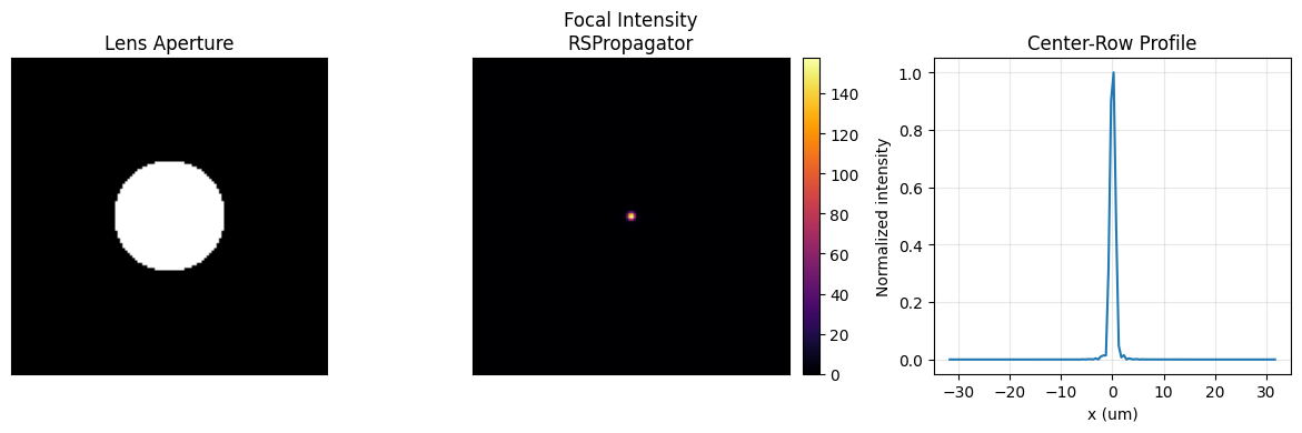
5 Plot Results#

The plots summarize the physical setup and result: the lens aperture, the focal-plane intensity, and a center-row intensity profile through the focused spot.

if PLOT:
    ARTIFACTS_DIR.mkdir(parents=True, exist_ok=True)
    fig, axes = plt.subplots(1, 3, figsize=(12.0, 3.8))

    axes[0].imshow(aperture_mask, cmap="gray")
    axes[0].set_title("Lens Aperture")
    axes[0].set_xticks([])
    axes[0].set_yticks([])

    focus_im = axes[1].imshow(intensity, cmap="inferno")
    axes[1].set_title(f"Focal Intensity\n{propagator.__class__.__name__}")
    axes[1].set_xticks([])
    axes[1].set_yticks([])
    plt.colorbar(focus_im, ax=axes[1], fraction=0.046, pad=0.04)

    axes[2].plot(x_um, center_row / np.maximum(np.max(center_row), 1e-12))
    axes[2].set_title("Center-Row Profile")
    axes[2].set_xlabel("x (um)")
    axes[2].set_ylabel("Normalized intensity")
    axes[2].grid(alpha=0.3)

    fig.tight_layout()
    fig.savefig(PLOT_PATH, dpi=150)
    plt.show()
    print(f"saved: {PLOT_PATH}")

../../_images/97be3ad69ee0649151233e1e8b70e07732a45014c74f6e9c7294ef4834795f3d.png

saved: /Users/liam/metasurface/fouriax/examples/artifacts/basic_propagation_overview.png