Diffractive Lens Optimization — Focusing a Plane Wave#
This notebook is the entry point for the lens-design family in the example set. It optimizes a single phase-only diffractive lens so a uniform plane wave forms a bright focal spot after free-space propagation.
Assumes you know#
basic coherent propagation and phase delay,
how intensity is computed from a propagated field, and
the idea of optimizing a differentiable optical system end to end.
New ideas in this notebook#
how to impose a circular aperture on a trainable phase element,
how a focal-spot loss turns wavefront design into a scalar optimization objective,
why the phase is bounded to \([0, 2\pi]\) during training, and
how the learned phase compares with the analytical hyperbolic phase of an ideal focusing lens.
Where to go next#
Continue to sensitivity_analysis.ipynb for measurement/design analysis of a lens, or to metaatom_optimization.ipynb for the same focusing task under a fabrication-library constraint.
0 Imports#
This notebook uses JAX and Optax for optimization, Matplotlib for diagnostics, and fouriax
primitives for the field, masks, propagation layer, and focal-spot loss.
from __future__ import annotations

from pathlib import Path

import jax
import jax.numpy as jnp
import matplotlib.pyplot as plt
import numpy as np
import optax

import fouriax as fx
%matplotlib inline

EXAMPLES_ROOT = Path.cwd() / "examples"
EXAMPLES_ARTIFACTS_DIR = EXAMPLES_ROOT / "artifacts"
1 Paths and Parameters#
The parameters define the simulation grid, wavelength, propagation distance, aperture diameter, and optimization workload. Together they specify both the optical problem and the optimization budget for maximizing intensity at the center pixel.
ARTIFACTS_DIR = Path(str(EXAMPLES_ARTIFACTS_DIR))
PLOT_PATH = ARTIFACTS_DIR / "lens_optimization_overview.png"
SUMMARY_PATH = ARTIFACTS_DIR / "lens_opt_summary.json"

SEED = 0
GRID_N = 64
GRID_DX_UM = 1.0
WAVELENGTH_UM = 0.532
DISTANCE_UM = 1000.0
APERTURE_DIAMETER_UM = 48.0
LR = 0.05
STEPS = 60
PLOT = True
2 Helper Functions#
The helper builds a binary circular aperture on the simulation grid. This separates two roles in the design:
the phase mask controls the wavefront, and
the aperture limits which pixels actually transmit light.
That distinction matters in later notebooks where the trainable surface is no longer an unconstrained phase map.
def circular_aperture(grid: fx.Grid, diameter_um: float) -> jnp.ndarray:
    x, y = grid.spatial_grid()
    r2 = x * x + y * y
    radius = diameter_um / 2.0
    return (r2 <= radius * radius).astype(jnp.float32)
3 Setup#
We illuminate the aperture with a plane wave, choose the center pixel as the desired focus, and build an optical module consisting of
The trainable parameter is an unconstrained array that is mapped through a sigmoid to a bounded phase mask, ensuring the learned optic remains phase-only throughout optimization.
grid = fx.Grid.from_extent(nx=GRID_N, ny=GRID_N, dx_um=GRID_DX_UM, dy_um=GRID_DX_UM)
spectrum = fx.Spectrum.from_scalar(WAVELENGTH_UM)
field_in = fx.Field.plane_wave(grid=grid, spectrum=spectrum)

aperture = circular_aperture(grid, diameter_um=APERTURE_DIAMETER_UM)
target_xy = (grid.nx // 2, grid.ny // 2)
propagator = fx.plan_propagation(
    mode="auto",
    grid=grid,
    spectrum=spectrum,
    distance_um=DISTANCE_UM,
)

def build_module(raw_phase_map: jnp.ndarray) -> fx.OpticalModule:
    phase_limited = 2.0 * jnp.pi * jax.nn.sigmoid(raw_phase_map)
    return fx.OpticalModule(
        layers=(
            fx.PhaseMask(phase_map_rad=phase_limited[None, :, :]),
            fx.AmplitudeMask(amplitude_map=aperture[None, :, :]),
            propagator,
        )
    )
4 Loss Function and Optimization#
The objective is the negative intensity at the center pixel, so minimizing it is equivalent to maximizing focused power at the optical axis. This turns the wave-optics design problem into a single scalar objective that Adam can optimize directly.
The optimizer keeps the best phase map encountered during training rather than assuming the final iterate is the best one.
def loss_fn(raw_phase_map: jnp.ndarray) -> jnp.ndarray:
    module = build_module(raw_phase_map)
    intensity = module.forward(field_in).intensity()
    center_intensity = intensity[..., target_xy[1], target_xy[0]]
    return -jnp.sum(center_intensity)

key = jax.random.PRNGKey(SEED)
phase_map = 0.1 * jax.random.normal(key, (grid.ny, grid.nx))

optimizer = optax.adam(LR)
result = fx.optim.optimize_optical_module(
    init_params=phase_map,
    build_module=build_module,
    loss_fn=loss_fn,
    optimizer=optimizer,
    steps=STEPS,
    log_every=20,
)
final_phase_limited = 2.0 * jnp.pi * jax.nn.sigmoid(result.best_params)
final_intensity = np.asarray(result.best_module.forward(field_in).intensity())[0]
optimized_profile = final_intensity[target_xy[1], :]
W0407 21:10:37.672346 1088181 cpp_gen_intrinsics.cc:74] Empty bitcode string provided for eigen. Optimizations relying on this IR will be disabled.
step=000 loss=-3.743369
step=020 loss=-11.184864
step=040 loss=-11.333426
step=059 loss=-11.405574
5 Evaluation#
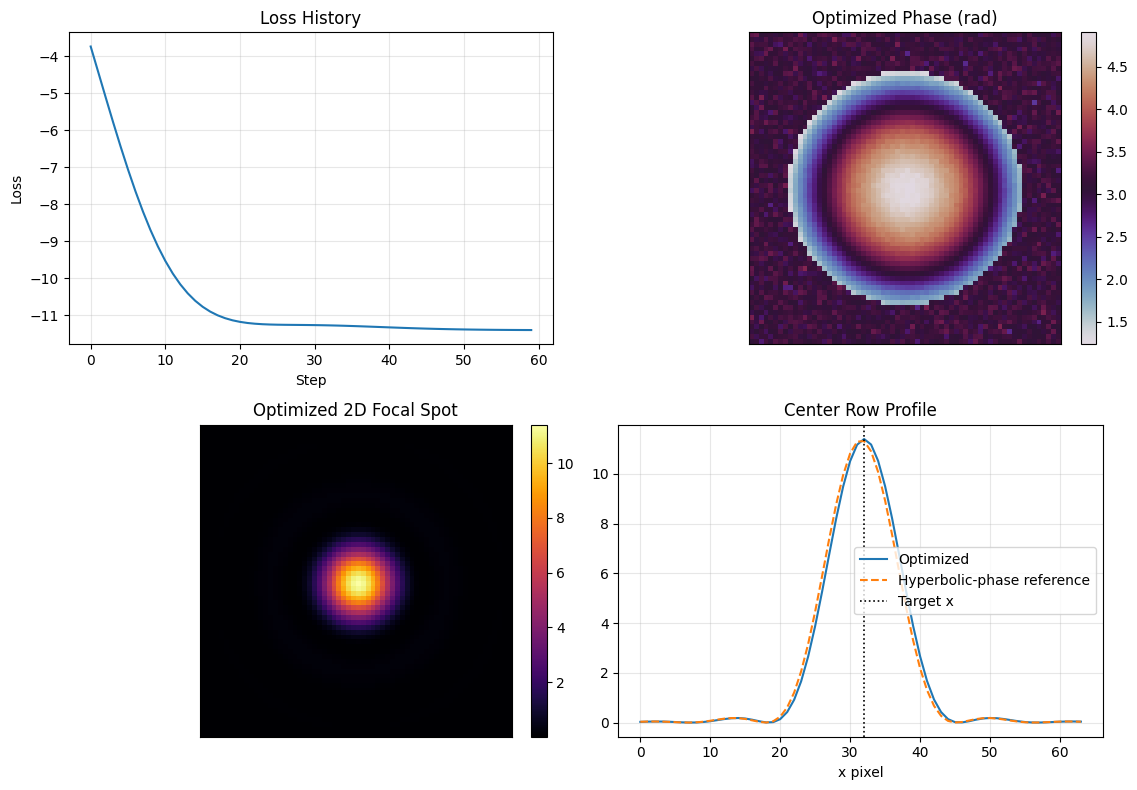
We compare the optimized lens against an analytical hyperbolic-phase reference with the same focal distance. The ideal reference phase used in the code is
which is the hyperbolic optical-path-delay profile for focusing a plane wave to distance \(f\). The comparison is intentionally simple: if the learned lens is behaving sensibly, its focal spot and center-row intensity profile should resemble the reference solution even though the training objective only asked for a bright focus.
x_um, y_um = grid.spatial_grid()
wavelength_um = float(spectrum.wavelengths_um[0])
k = 2.0 * jnp.pi / wavelength_um
hyperbolic_phase = -k * (jnp.sqrt(x_um * x_um + y_um * y_um + DISTANCE_UM**2) - DISTANCE_UM)
reference_module = fx.OpticalModule(
    layers=(
        fx.PhaseMask(phase_map_rad=hyperbolic_phase[None, :, :]),
        fx.AmplitudeMask(amplitude_map=aperture[None, :, :]),
        propagator,
    )
)
reference_intensity = np.asarray(reference_module.forward(field_in).intensity())[0]
reference_profile = reference_intensity[target_xy[1], :]
6 Plot Results#
The overview figure combines optimization dynamics, the learned phase pattern, the 2D focal spot, and a 1D profile comparison against the analytical lens.
The key interpretation is not that the learned phase must numerically equal the hyperbolic phase at every pixel, but that it should produce a similarly concentrated focus at the target location.
if PLOT:
    optimized_phase = np.asarray(final_phase_limited)
    fig, axes = plt.subplots(2, 2, figsize=(11.5, 8.0))

    axes[0, 0].plot(result.history)
    axes[0, 0].set_title("Loss History")
    axes[0, 0].set_xlabel("Step")
    axes[0, 0].set_ylabel("Loss")
    axes[0, 0].grid(alpha=0.3)

    phase_im = axes[0, 1].imshow(optimized_phase, cmap="twilight")
    axes[0, 1].set_title("Optimized Phase (rad)")
    axes[0, 1].set_xticks([])
    axes[0, 1].set_yticks([])
    plt.colorbar(phase_im, ax=axes[0, 1], fraction=0.046, pad=0.04)

    focus_im = axes[1, 0].imshow(final_intensity, cmap="inferno")
    axes[1, 0].set_title("Optimized 2D Focal Spot")
    axes[1, 0].set_xticks([])
    axes[1, 0].set_yticks([])
    plt.colorbar(focus_im, ax=axes[1, 0], fraction=0.046, pad=0.04)

    axes[1, 1].plot(optimized_profile, label="Optimized")
    axes[1, 1].plot(reference_profile, label="Hyperbolic-phase reference", linestyle="--")
    axes[1, 1].axvline(
        target_xy[0], color="black", linestyle=":", linewidth=1.2, label="Target x"
    )
    axes[1, 1].set_title("Center Row Profile")
    axes[1, 1].set_xlabel("x pixel")
    axes[1, 1].grid(alpha=0.3)
    axes[1, 1].legend()

    fig.tight_layout()
    fig.savefig(PLOT_PATH, dpi=150)
    plt.show()
    print(f"saved: {PLOT_PATH}")
saved: /Users/liam/metasurface/fouriax/examples/artifacts/lens_optimization_overview.png