Meta-Atom Library Optimization — Focusing with Interpolated Unit Cells#
This notebook is the fabrication-constrained child notebook in the lens-design family. It builds on lens_optimization.ipynb: the optical goal is still to focus a plane wave, but the trainable surface is now restricted to a meta-atom library rather than an arbitrary phase mask.
Assumes you know#
the focusing setup from lens_optimization.ipynb,
why a hyperbolic phase profile is the natural focusing reference, and
the basics of optimizing a differentiable optical module.
What changes relative to the parent notebook#
each pixel is parameterized by a bounded geometry variable instead of a free phase,
optical transmission comes from interpolating a precomputed meta-atom lookup table, and
the design is limited to what the unit-cell library can physically realize.
The parent notebook covers the focusing intuition; this notebook focuses on what changes when fabrication constraints are part of the model.
0 Imports#
The imports look similar to the parent lens notebook, but the core new dependency is the meta-atom
library interface in fouriax, used to turn geometry parameters into complex transmission values.
from __future__ import annotations

from pathlib import Path

import jax
import jax.numpy as jnp
import matplotlib.pyplot as plt
import numpy as np
import optax

import fouriax as fx
%matplotlib inline

EXAMPLES_ROOT = Path.cwd() / "examples"
EXAMPLES_DATA_DIR = EXAMPLES_ROOT / "data"
EXAMPLES_ARTIFACTS_DIR = EXAMPLES_ROOT / "artifacts"
1 Paths and Parameters#
Besides the usual artifact path and optimization settings, this notebook introduces the NPZ lookup-table path and the selected wavelength used to slice the library. Those settings determine which physical library and operating point the optimizer is allowed to use.
NPZ_PATH = Path(str(EXAMPLES_DATA_DIR / 'meta_atoms' / 'square_pillar_0p7um_cell_sweep_results.npz'))
ARTIFACTS_DIR = Path(str(EXAMPLES_ARTIFACTS_DIR))
PLOT_PATH = ARTIFACTS_DIR / "metaatom_opt_overview.png"
SUMMARY_PATH = ARTIFACTS_DIR / "metaatom_opt_summary.json"

SPEED_OF_LIGHT_M_PER_S = 299792458.0
SEED = 0
GRID_N = 64
GRID_DX_UM = 0.7
SELECTED_WAVELENGTH_UM = 1.3
DISTANCE_UM = 100.0
LR = 0.1
STEPS = 180
PLOT = True
2 Helper Functions#
The helper loads the square-pillar sweep data, sorts the wavelength and geometry axes, and converts transmission magnitude and phase into a complex meta-atom library. This is the interface between an external electromagnetic sweep and the differentiable optical model used here.
def load_square_pillar_library(npz_path: Path) -> fx.MetaAtomLibrary:
    """Load LUT from NPZ keys: freqs [Hz], side_lengths [m], trans, phase."""
    with np.load(npz_path) as data:
        freqs_hz = np.asarray(data["freqs"], dtype=np.float64).reshape(-1)
        side_lengths_m = np.asarray(data["side_lengths"], dtype=np.float64).reshape(-1)
        trans = np.asarray(data["trans"], dtype=np.float64)
        phase = np.asarray(data["phase"], dtype=np.float64)

    wavelengths_um = (SPEED_OF_LIGHT_M_PER_S / freqs_hz) * 1e6
    side_lengths_um = side_lengths_m * 1e6

    wav_order = np.argsort(wavelengths_um)
    side_order = np.argsort(side_lengths_um)

    wavelengths_um = wavelengths_um[wav_order]
    side_lengths_um = side_lengths_um[side_order]

    trans = trans[side_order, :][:, wav_order]
    phase = phase[side_order, :][:, wav_order]

    transmission_complex = trans.T * np.exp(1j * phase.T)

    return fx.MetaAtomLibrary.from_complex(
        wavelengths_um=jnp.asarray(wavelengths_um, dtype=jnp.float32),
        parameter_axes=(jnp.asarray(side_lengths_um, dtype=jnp.float32),),
        transmission_complex=jnp.asarray(transmission_complex),
    )
3 Setup#
We choose the library wavelength closest to the requested operating wavelength, construct the working
grid, and build an optical module whose first layer is MetaAtomInterpolationLayer.
Unlike the parent notebook, the trainable parameter is now a geometry map bounded between the minimum and maximum side lengths present in the library. The propagation target is still the central focal spot.
library = load_square_pillar_library(NPZ_PATH)

nearest_idx = int(jnp.argmin(jnp.abs(library.wavelengths_um - SELECTED_WAVELENGTH_UM)))
wavelength_um = float(library.wavelengths_um[nearest_idx])
grid = fx.Grid.from_extent(nx=GRID_N, ny=GRID_N, dx_um=GRID_DX_UM, dy_um=GRID_DX_UM)
spectrum = fx.Spectrum.from_scalar(wavelength_um)
field_in = fx.Field.plane_wave(grid=grid, spectrum=spectrum)

target_xy = (grid.nx // 2, grid.ny // 2)
propagator = fx.plan_propagation(
    mode="auto",
    grid=grid,
    spectrum=spectrum,
    distance_um=DISTANCE_UM,
)

side_axis = library.parameter_axes[0]
min_bounds = jnp.array([side_axis[0]], dtype=jnp.float32)
max_bounds = jnp.array([side_axis[-1]], dtype=jnp.float32)

def build_module(raw_params: jnp.ndarray) -> fx.OpticalModule:
    return fx.OpticalModule(
        layers=(
            fx.MetaAtomInterpolationLayer(
                library=library,
                raw_geometry_params=raw_params,
                min_geometry_params=min_bounds,
                max_geometry_params=max_bounds,
            ),
            propagator,
        )
    )
4 Loss Function and Optimization#
The loss is deliberately minimal: maximize the on-axis focal intensity by minimizing its negative. The optimizer therefore searches over physically realizable unit-cell geometries rather than over a free phase profile.
This makes the comparison to the parent notebook meaningful: the optical task is the same, but the design space is much narrower and more realistic.
def loss_fn(raw_params: jnp.ndarray) -> jnp.ndarray:
    module = build_module(raw_params)
    intensity = module.forward(field_in).intensity()
    center = intensity[0, target_xy[1], target_xy[0]]
    return -center

key = jax.random.PRNGKey(SEED)
raw_params = 0.1 * jax.random.normal(key, (grid.ny, grid.nx), dtype=jnp.float32)
optimizer = optax.adam(learning_rate=LR)

result = fx.optim.optimize_optical_module(
    init_params=raw_params,
    build_module=build_module,
    loss_fn=loss_fn,
    optimizer=optimizer,
    steps=STEPS,
    log_every=30,
)
W0407 21:10:54.919071 1088538 cpp_gen_intrinsics.cc:74] Empty bitcode string provided for eigen. Optimizations relying on this IR will be disabled.
step=000 loss=-0.516717
step=030 loss=-75.398956
step=060 loss=-83.244080
step=090 loss=-85.687599
step=120 loss=-86.851814
step=150 loss=-87.272255
step=179 loss=-87.786316
5 Evaluation#
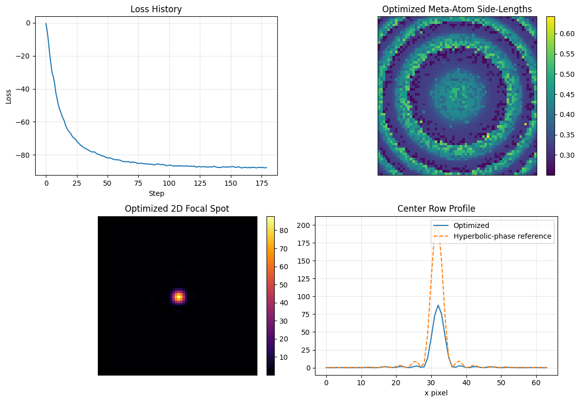
We evaluate the best library-constrained design against the same hyperbolic-phase reference used in lens_optimization.ipynb. In addition to the focal intensity profile, we can now inspect the optimized side-length map, which is the actual fabrication-facing output of the optimization.
final_intensity = np.asarray(result.best_module.forward(field_in).intensity())
optimized_profile = final_intensity[0, target_xy[1], :]

# Reference: phase profile for ideal spherical wavefront convergence at distance_um.
x_um, y_um = grid.spatial_grid()
k = 2.0 * jnp.pi / wavelength_um
hyperbolic_phase = -k * (jnp.sqrt(x_um * x_um + y_um * y_um + DISTANCE_UM**2) - DISTANCE_UM)
reference_module = fx.OpticalModule(
    layers=(
        fx.PhaseMask(phase_map_rad=hyperbolic_phase[None, :, :]),
        propagator,
    )
)

reference_intensity = np.asarray(reference_module.forward(field_in).intensity())
reference_profile = reference_intensity[0, target_xy[1], :]

final_layer = fx.MetaAtomInterpolationLayer(
    library=library,
    raw_geometry_params=result.best_params,
    min_geometry_params=min_bounds,
    max_geometry_params=max_bounds,
)
optimized_side_map = np.asarray(final_layer.bounded_geometry_params()[0])
6 Plot Results#
The figure shows whether the constrained design still focuses well, what geometry map the optimizer settled on, and how its focal profile compares with the ideal phase-only reference.
Interpret the result as a tradeoff plot: if the focus remains sharp while the geometry map stays inside the library bounds, the meta-atom parameterization is expressive enough for this task.
if PLOT:
    fig, axes = plt.subplots(2, 2, figsize=(11.5, 8.0))

    axes[0, 0].plot(result.history)
    axes[0, 0].set_title("Loss History")
    axes[0, 0].set_xlabel("Step")
    axes[0, 0].set_ylabel("Loss")
    axes[0, 0].grid(alpha=0.3)

    side_im = axes[0, 1].imshow(optimized_side_map, cmap="viridis")
    axes[0, 1].set_title("Optimized Meta-Atom Side-Lengths")
    axes[0, 1].set_xticks([])
    axes[0, 1].set_yticks([])
    plt.colorbar(side_im, ax=axes[0, 1], fraction=0.046, pad=0.04)

    focus_im = axes[1, 0].imshow(final_intensity[0], cmap="inferno")
    axes[1, 0].set_title("Optimized 2D Focal Spot")
    axes[1, 0].set_xticks([])
    axes[1, 0].set_yticks([])
    plt.colorbar(focus_im, ax=axes[1, 0], fraction=0.046, pad=0.04)

    axes[1, 1].plot(optimized_profile, label="Optimized")
    axes[1, 1].plot(reference_profile, label="Hyperbolic-phase reference", linestyle="--")
    axes[1, 1].set_title("Center Row Profile")
    axes[1, 1].set_xlabel("x pixel")
    axes[1, 1].grid(alpha=0.3)
    axes[1, 1].legend()

    fig.tight_layout()
    fig.savefig(PLOT_PATH, dpi=150)
    plt.show()
    print(f"saved: {PLOT_PATH}")
saved: /Users/liam/metasurface/fouriax/examples/artifacts/metaatom_opt_overview.png