Sensitivity Analysis and Fisher Information for a Diffractive Lens#
This notebook is the analysis child notebook in the lens-design family. It builds on the same focusing setup introduced in lens_optimization.ipynb, but shifts the question from design to diagnosis: how informative is the focal-plane measurement, and which phase pixels matter most to the output?
Assumes you know#
the lens-style focusing problem from lens_optimization.ipynb,
how a phase mask and propagation layer produce a focal intensity pattern, and
basic matrix/Jacobian notation.
What changes relative to the parent notebook#
the phase mask is fixed rather than optimized,
we evaluate the output as a measurement model for incident angle estimation, and
we compute design sensitivity and a simple fabrication-tolerance map from output Jacobians.
This notebook does not repeat the focusing derivation; it focuses on what can be learned about a lens once a nominal design is already in hand.
0 Imports#
We use NumPy and Matplotlib for reporting, together with fouriax.analysis helpers for Fisher
information, Cramér-Rao bounds, D-optimality, and sensitivity maps.
from __future__ import annotations

from pathlib import Path

import jax.numpy as jnp
import matplotlib.pyplot as plt
import numpy as np

import fouriax as fx
%matplotlib inline

EXAMPLES_ROOT = Path.cwd() / "examples"
EXAMPLES_ARTIFACTS_DIR = EXAMPLES_ROOT / "artifacts"
1 Paths and Parameters#
The parameters define a nominal focusing geometry plus two analysis-specific knobs:
the off-axis angle to be estimated in the Fisher-information study, and
the pooling factor used to keep the design-sensitivity Jacobian tractable.
These control the statistical and computational scales of the analysis rather than a training loop.
ARTIFACTS_DIR = Path(str(EXAMPLES_ARTIFACTS_DIR))
PLOT_PATH = ARTIFACTS_DIR / "sensitivity_analysis_overview.png"

SEED = 0
GRID_N = 32
GRID_DX_UM = 1.0
WAVELENGTH_UM = 0.532
DISTANCE_UM = 150.0
NOMINAL_ANGLE_RAD = 0.005
NOMINAL_DIRECTION_DEG = 0.0
STRETCH_FACTOR = 1.5
INPUT_COUNT_SCALE = 1000.0
SENSITIVITY_POOL = 4
PLOT = True
2 Helper Functions#
The helper functions define the nominal stretched hyperbolic phase mask and the pooled output metric used for sensitivity analysis. Pooling is a pragmatic numerical choice: it reduces the output dimension before Jacobians are formed, which substantially lowers memory use without changing the qualitative interpretation of the sensitivity map.
def stretched_hyperbolic_phase(
    grid: fx.Grid,
    distance_um: float,
    wavelength_um: float,
    stretch_factor: float = 2.0,
) -> jnp.ndarray:
    x, y = grid.spatial_grid()
    k = 2.0 * jnp.pi / wavelength_um
    return -k * (jnp.sqrt(stretch_factor * x * x + y * y + distance_um**2) - distance_um)


def pooled_metric(image: jnp.ndarray, pool: int) -> jnp.ndarray:
    if pool <= 1:
        return image.ravel()
    if image.shape[0] % pool != 0 or image.shape[1] % pool != 0:
        raise ValueError(
            "sensitivity_pool must divide both image dimensions; "
            f"got pool={pool} for shape={image.shape}"
        )
    pooled = image.reshape(
        image.shape[0] // pool,
        pool,
        image.shape[1] // pool,
        pool,
    ).mean(axis=(1, 3))
    return pooled.ravel()
3 Setup#
We build a fixed phase-mask lens and a plane-wave input field with configurable photon-count scale. The phase profile is intentionally anisotropic through the stretch factor so the downstream analysis has nontrivial spatial structure to reveal.
if SENSITIVITY_POOL <= 0:
    raise ValueError("sensitivity_pool must be strictly positive")
grid = fx.Grid.from_extent(nx=GRID_N, ny=GRID_N, dx_um=GRID_DX_UM, dy_um=GRID_DX_UM)
spectrum = fx.Spectrum.from_scalar(WAVELENGTH_UM)
propagator = fx.plan_propagation(
    mode="auto",
    grid=grid,
    spectrum=spectrum,
    distance_um=DISTANCE_UM,
)

# Use a hyperbolic lens phase as the "optimized" design
phase = stretched_hyperbolic_phase(grid, DISTANCE_UM, WAVELENGTH_UM, STRETCH_FACTOR)

def make_module(phase_map: jnp.ndarray) -> fx.OpticalModule:
    return fx.OpticalModule(
        layers=(
            fx.PhaseMask(phase_map_rad=phase_map[None, :, :]),
            propagator,
        )
    )

input_amp = jnp.sqrt(jnp.asarray(INPUT_COUNT_SCALE, dtype=jnp.float32))
field_in = fx.Field.plane_wave(grid=grid, spectrum=spectrum, amplitude=input_amp)

def forward_intensity(phase_map: jnp.ndarray) -> jnp.ndarray:
    return make_module(phase_map).forward(field_in).intensity()[0]
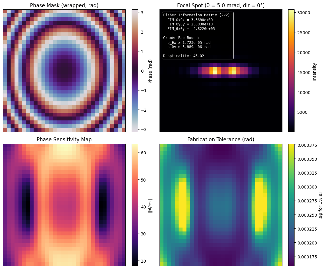
4 Observation Fisher Information (angle of incidence)#
Here the lens is treated as part of a statistical forward model \( (\theta_x, \theta_y) \mapsto I(x,y) \). We compute the Fisher Information Matrix for a nominal incident angle under Poisson noise, then derive the corresponding Cramér-Rao bound and D-optimality.
If \(\mu(\theta) \in \mathbb{R}^m\) is the predicted intensity vector and
\(J(\theta) = \partial \mu / \partial \theta\) is its Jacobian, then the closed-form Fisher matrix used
by fouriax.analysis.fisher_information() is
where \(\Lambda\) is the noise precision matrix. For independent Poisson counts, \(\Lambda(\theta) = \mathrm{diag}(1/\mu_i(\theta))\), so elementwise
The D-optimality score used here is the log-determinant criterion
which increases as the measurement becomes more informative in all parameter directions.
This section answers a measurement question: how precisely could this focal-plane intensity pattern, in principle, estimate small changes in input angle?
k = 2.0 * jnp.pi / WAVELENGTH_UM
x_grid, y_grid = grid.spatial_grid()

def forward_angle(angles: jnp.ndarray) -> jnp.ndarray:
    """Map (θ_x, θ_y) → focal-plane intensity."""
    theta_x, theta_y = angles[0], angles[1]
    tilt_phase = k * (theta_x * x_grid + theta_y * y_grid)
    field_data = (input_amp * jnp.exp(1j * tilt_phase)).astype(jnp.complex64)
    field_tilted = fx.Field(
        data=field_data[None, :, :],
        grid=grid,
        spectrum=spectrum,
        domain="spatial",
    )
    return make_module(phase).forward(field_tilted).intensity()[0].ravel()

# Off-axis nominal angle at the configured direction
angle_dir = jnp.deg2rad(NOMINAL_DIRECTION_DEG)
angles_nominal = NOMINAL_ANGLE_RAD * jnp.array(
    [jnp.cos(angle_dir), jnp.sin(angle_dir)],
)
print("Computing observation FIM (angle of incidence)...")
fim_angle = fx.analysis.fisher_information(
    forward_angle,
    angles_nominal,
    noise_model=fx.PoissonNoise(count_scale=1.0),
)
crb_angle = fx.analysis.cramer_rao_bound(fim_angle, regularize=1e-15)
d_opt = fx.analysis.d_optimality(fim_angle)

fim_np = np.asarray(fim_angle)
crb_np = np.asarray(crb_angle)
print(f"FIM (2×2):\n{fim_np}")
print(f"CRB (θ_x, θ_y): ({crb_np[0]:.3e}, {crb_np[1]:.3e}) rad²")
print(
    f"Angular precision: σ_θx={np.sqrt(max(crb_np[0], 0)):.3e}, "
    f"σ_θy={np.sqrt(max(crb_np[1], 0)):.3e} rad"
)
print(f"D-optimality: {float(d_opt):.2f}")
Computing observation FIM (angle of incidence)...
FIM (2×2):
[[ 3.3679982e+09 -4.8226044e+05]
 [-4.8231772e+05  2.8830220e+10]]
CRB (θ_x, θ_y): (2.969e-10, 3.469e-11) rad²
Angular precision: σ_θx=1.723e-05, σ_θy=5.889e-06 rad
D-optimality: 46.02
5 Design Sensitivity Analysis#
We now switch from parameter estimation to device robustness. The sensitivity map measures how much the chosen output metric changes when each phase pixel is perturbed, while the tolerance map inverts that quantity into an approximate allowable phase error for a 1% output change.
If \(m(I)\) is the chosen output metric and \(\phi_j\) is the \(j\)th phase parameter, the Jacobian-based
sensitivity reported by fouriax.analysis.sensitivity_map() is the column norm
Using the first-order approximation in parameter_tolerance(), the allowable perturbation for a
target metric change \(\varepsilon\) is
In this notebook we use \(\varepsilon = 0.01\), corresponding to an approximate 1% output change.
High sensitivity means a pixel is optically important but fabrication-critical; high tolerance means the design is comparatively forgiving there.
print("Computing design sensitivity (per-pixel phase sensitivity)...")
def metric_fn(output: jnp.ndarray) -> jnp.ndarray:
    return pooled_metric(output, SENSITIVITY_POOL)

sens = fx.analysis.sensitivity_map(forward_intensity, phase, metric_fn=metric_fn)
sens_np = np.asarray(sens)

print("Computing fabrication tolerance map...")
tol = 0.01 / jnp.maximum(sens, 1e-12)
tol_np = np.asarray(tol)
Computing design sensitivity (per-pixel phase sensitivity)...
Computing fabrication tolerance map...
6 Plot Results#
The final figure combines the nominal phase design, the off-axis focal pattern with its Fisher statistics, the spatial sensitivity map, and the derived tolerance map.
Read these panels together: the notebook is most useful when it tells you not only that a lens works, but also which measurements it supports well and which regions of the design are fragile to phase errors.
if PLOT:
    ARTIFACTS_DIR.mkdir(parents=True, exist_ok=True)

    fig, axes = plt.subplots(2, 2, figsize=(11.5, 9.0))

    phase_wrapped = np.angle(np.exp(1j * np.asarray(phase)))
    im0 = axes[0, 0].imshow(phase_wrapped, cmap="twilight", vmin=-np.pi, vmax=np.pi)
    axes[0, 0].set_title("Phase Mask (wrapped, rad)")
    axes[0, 0].set_xticks([])
    axes[0, 0].set_yticks([])
    plt.colorbar(im0, ax=axes[0, 0], fraction=0.046, pad=0.04, label="Phase (rad)")

    intensity = np.asarray(
        forward_angle(angles_nominal).reshape(GRID_N, GRID_N),
    )
    im1 = axes[0, 1].imshow(intensity, cmap="inferno")
    theta_mrad = float(NOMINAL_ANGLE_RAD * 1e3)
    axes[0, 1].set_title(
        f"Focal Spot (θ = {theta_mrad:.1f} mrad, dir = {NOMINAL_DIRECTION_DEG:.0f}°)",
    )
    axes[0, 1].set_xticks([])
    axes[0, 1].set_yticks([])
    plt.colorbar(im1, ax=axes[0, 1], fraction=0.046, pad=0.04, label="Intensity")
    axes[0, 1].text(
        0.03,
        0.97,
        (
            f"Fisher Information Matrix (2×2):\n"
            f"  FIM_θxθx = {fim_np[0, 0]:.4e}\n"
            f"  FIM_θyθy = {fim_np[1, 1]:.4e}\n"
            f"  FIM_θxθy = {fim_np[0, 1]:.4e}\n\n"
            f"Cramér–Rao Bound:\n"
            f"  σ_θx ≥ {np.sqrt(max(crb_np[0], 0)):.3e} rad\n"
            f"  σ_θy ≥ {np.sqrt(max(crb_np[1], 0)):.3e} rad\n\n"
            f"D-optimality: {float(d_opt):.2f}"
        ),
        transform=axes[0, 1].transAxes,
        va="top",
        ha="left",
        fontsize=8.5,
        family="monospace",
        color="white",
        bbox={
            "boxstyle": "round,pad=0.35",
            "facecolor": "black",
            "alpha": 0.70,
            "edgecolor": "white",
            "linewidth": 0.8,
        },
    )

    im2 = axes[1, 0].imshow(sens_np, cmap="magma")
    axes[1, 0].set_title("Phase Sensitivity Map")
    axes[1, 0].set_xticks([])
    axes[1, 0].set_yticks([])
    plt.colorbar(im2, ax=axes[1, 0], fraction=0.046, pad=0.04, label="‖∂I/∂φᵢ‖")

    tol_clipped = np.clip(tol_np, 0, np.nanpercentile(tol_np, 95))
    im3 = axes[1, 1].imshow(tol_clipped, cmap="viridis")
    axes[1, 1].set_title("Fabrication Tolerance (rad)")
    axes[1, 1].set_xticks([])
    axes[1, 1].set_yticks([])
    plt.colorbar(im3, ax=axes[1, 1], fraction=0.046, pad=0.04, label="Δφ for 1% ΔI")

    fig.tight_layout()
    fig.savefig(PLOT_PATH, dpi=150)
    plt.show()
    print(f"saved: {PLOT_PATH}")
saved: /Users/liam/metasurface/fouriax/examples/artifacts/sensitivity_analysis_overview.png