Polarization-Multiplexed Holography — Dual Reconstructions#
This notebook is the holography extension notebook. It builds directly on hologram_coherent_logo.ipynb: the propagation problem is the same, but the optical element is now a Jones-matrix hologram that sends different images to the two linear polarization components.
Assumes you know#
the phase-only holography setup from hologram_coherent_logo.ipynb,
how normalized intensity matching is used as the reconstruction loss, and
the basics of Jones-vector polarization notation.
What changes relative to the parent notebook#
the input field carries both
xandypolarization components,the hologram is a diagonal Jones matrix rather than a scalar phase mask, and
the loss supervises two reconstructions at once, one per polarization channel.
The parent notebook covers the phase-only holography intuition, so this notebook focuses only on the polarization-specific delta.
0 Imports#
The imports match the single-channel hologram notebook, with the same JAX/Optax optimization stack
and PIL image loading. The new ingredient is not a new dependency, but a different fouriax
optical layer: JonesMatrixLayer.
from __future__ import annotations

from pathlib import Path

import jax
import jax.numpy as jnp
import matplotlib.pyplot as plt
import numpy as np
import optax
from PIL import Image

import fouriax as fx
%matplotlib inline

EXAMPLES_ROOT = Path.cwd() / "examples"
EXAMPLES_DATA_DIR = EXAMPLES_ROOT / "data"
EXAMPLES_ARTIFACTS_DIR = EXAMPLES_ROOT / "artifacts"
1 Paths and Parameters#
The grid, wavelength, propagation distance, and optimization settings mirror the scalar hologram example so the change in behavior can be attributed to polarization multiplexing rather than a new numerical regime.
IMAGE_PATH = Path(str(EXAMPLES_DATA_DIR / 'logo.jpg'))
ARTIFACTS_DIR = Path(str(EXAMPLES_ARTIFACTS_DIR))
PLOT_PATH = ARTIFACTS_DIR / "holography_polarized_dual_overview.png"

SEED = 0
NX = 128
NY = 128
DX_UM = 1.0
DY_UM = 1.0
WAVELENGTH_UM = 0.532
DISTANCE_UM = 1200.0
NYQUIST_FACTOR = 2.0
MIN_PADDING_FACTOR = 2.0
STEPS = 400
LR = 0.03
PLOT = True
2 Helper Functions#
We reuse the same logo-to-binary-mask conversion as the parent notebook. The second target is then created by rotating the first one by \(180^\circ\), giving the two polarization channels clearly separable objectives.
def load_logo_target(path: Path, grid: fx.Grid) -> jnp.ndarray:
    """Load image and convert to binary target: white->0, red-logo->1."""
    img = Image.open(path).convert("RGB").resize((grid.nx, grid.ny), Image.Resampling.BILINEAR)
    rgb = np.asarray(img, dtype=np.float32) / 255.0
    r = rgb[..., 0]
    g = rgb[..., 1]
    b = rgb[..., 2]
    red_mask = (r >= 0.55) & (g <= 0.45) & (b <= 0.45)
    return jnp.asarray(red_mask.astype(np.float32), dtype=jnp.float32)
3 Setup#
The input is now a Jones field with both E_x and E_y present. The trainable optic is a
pixelwise diagonal Jones matrix
so the two polarization channels see different phase delays while remaining uncoupled.
This is the key difference from the parent notebook: one physical surface carries two phase maps, one for each polarization basis component.
if not IMAGE_PATH.exists():
    raise FileNotFoundError(f"image not found: {IMAGE_PATH}")

grid = fx.Grid.from_extent(nx=NX, ny=NY, dx_um=DX_UM, dy_um=DY_UM)
base_target = load_logo_target(IMAGE_PATH, grid=grid)
target_x = base_target
target_y = jnp.rot90(base_target, k=2, axes=(0, 1))

spectrum = fx.Spectrum.from_scalar(WAVELENGTH_UM)

field_in = fx.Field.plane_wave_jones(
    grid=grid,
    spectrum=spectrum,
    ex=1.0 + 0.0j,
    ey=1.0 + 0.0j,
)
propagator = fx.plan_propagation(
    mode="auto",
    grid=grid,
    spectrum=spectrum,
    distance_um=DISTANCE_UM,
    nyquist_factor=NYQUIST_FACTOR,
    min_padding_factor=MIN_PADDING_FACTOR,
)

def build_module(raw_phase: jnp.ndarray) -> fx.OpticalModule:
    phase = 2.0 * jnp.pi * jax.nn.sigmoid(raw_phase)
    jxx = jnp.exp(1j * phase[0]).astype(jnp.complex64)
    jyy = jnp.exp(1j * phase[1]).astype(jnp.complex64)
    zeros = jnp.zeros_like(jxx)
    jones = jnp.stack(
        [
            jnp.stack([jxx, zeros], axis=0),
            jnp.stack([zeros, jyy], axis=0),
        ],
        axis=0,
    )
    return fx.OpticalModule(
        layers=(
            fx.JonesMatrixLayer(jones_matrix=jones),
            propagator,
        )
    )
4 Loss Function and Optimization#
The loss propagates the Jones field, extracts the per-component intensities, normalizes each one
independently, and matches them to target_x and target_y.
Training therefore asks a stronger question than the scalar hologram example: can one shared device encode two independent images when read through polarization analysis?
def loss_fn(raw_phase: jnp.ndarray) -> jnp.ndarray:
    module = build_module(raw_phase)
    out = module.forward(field_in)
    component_intensity = out.component_intensity()[0]
    ix = component_intensity[0]
    iy = component_intensity[1]
    ix_norm = ix / jnp.maximum(jnp.max(ix), 1e-12)
    iy_norm = iy / jnp.maximum(jnp.max(iy), 1e-12)
    return jnp.mean((ix_norm - target_x) ** 2) + jnp.mean((iy_norm - target_y) ** 2)

key = jax.random.PRNGKey(SEED)
raw_phase = 0.1 * jax.random.normal(key, (2, grid.ny, grid.nx), dtype=jnp.float32)
optimizer = optax.adam(LR)
result = fx.optim.optimize_optical_module(
    init_params=raw_phase,
    build_module=build_module,
    loss_fn=loss_fn,
    optimizer=optimizer,
    steps=STEPS,
    log_every=50,
)
W0407 21:02:40.191301 1082889 cpp_gen_intrinsics.cc:74] Empty bitcode string provided for eigen. Optimizations relying on this IR will be disabled.
step=000 loss=0.474987
step=050 loss=0.198434
step=100 loss=0.144278
step=150 loss=0.065695
step=200 loss=0.040990
step=250 loss=0.035248
step=300 loss=0.032215
step=350 loss=0.029542
step=399 loss=0.027540
5 Evaluation#
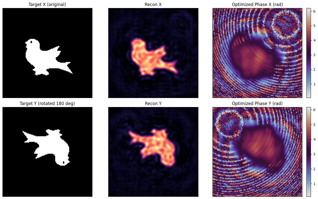
After optimization, we convert the best raw parameters into the two physical phase maps \(\phi_x\) and \(\phi_y\), then inspect the reconstructed intensities for both polarization channels. This separates device design from readout: the figure shows what each analyzed component would produce at the output plane.
phase_opt = 2.0 * jnp.pi * jax.nn.sigmoid(result.best_params)
out_opt = result.best_module.forward(field_in)
component_intensity = out_opt.component_intensity()[0]
recon_x = component_intensity[0]
recon_y = component_intensity[1]
recon_x_norm = recon_x / jnp.maximum(jnp.max(recon_x), 1e-12)
recon_y_norm = recon_y / jnp.maximum(jnp.max(recon_y), 1e-12)

ARTIFACTS_DIR.mkdir(parents=True, exist_ok=True)
6 Plot Results#
The top row reports the x-polarized target, reconstruction, and learned phase; the bottom row does
the same for the y channel. Success here means each polarization component reproduces its own
pattern without simply duplicating the other one.
The result demonstrates the main point of polarization multiplexing: the same pixel grid can carry multiple holographic functions when the field has additional internal degrees of freedom.
if PLOT:
    fig, axes = plt.subplots(2, 3, figsize=(13, 8))
    axes[0, 0].imshow(np.asarray(target_x), cmap="gray", vmin=0.0, vmax=1.0)
    axes[0, 0].set_title("Target X (original)")
    axes[0, 1].imshow(np.asarray(recon_x_norm), cmap="magma", vmin=0.0, vmax=1.0)
    axes[0, 1].set_title("Recon X")
    sx_im = axes[0, 2].imshow(np.asarray(phase_opt[0]), cmap="twilight")
    axes[0, 2].set_title("Optimized Phase X (rad)")
    plt.colorbar(sx_im, ax=axes[0, 2], fraction=0.046, pad=0.04)

    axes[1, 0].imshow(np.asarray(target_y), cmap="gray", vmin=0.0, vmax=1.0)
    axes[1, 0].set_title("Target Y (rotated 180 deg)")
    axes[1, 1].imshow(np.asarray(recon_y_norm), cmap="magma", vmin=0.0, vmax=1.0)
    axes[1, 1].set_title("Recon Y")
    sy_im = axes[1, 2].imshow(np.asarray(phase_opt[1]), cmap="twilight")
    axes[1, 2].set_title("Optimized Phase Y (rad)")
    plt.colorbar(sy_im, ax=axes[1, 2], fraction=0.046, pad=0.04)

    for ax in axes.flatten():
        ax.set_xticks([])
        ax.set_yticks([])
    fig.tight_layout()
    fig.savefig(PLOT_PATH, dpi=150)
    plt.show()
    print(f"saved: {PLOT_PATH}")
saved: /Users/liam/metasurface/fouriax/examples/artifacts/holography_polarized_dual_overview.png