Coherent Hologram — Phase-Only Logo Reconstruction#
This notebook is the entry point for the holography family in the example set. It shows the simplest coherent holography task here: learn a single phase-only mask so a uniform incident field reconstructs a binary logo after free-space propagation.
Assumes you know#
basic coherent propagation and complex fields,
how intensity is measured from a propagated field, and
the idea of gradient-based optimization in JAX.
New ideas in this notebook#
why phase-only control can still shape an intensity pattern after propagation,
how to turn a colored input image into a binary holography target,
why the loss is computed on normalized intensity rather than raw power, and
how
plan_propagation()chooses a numerically safe propagator and padding regime.
Where to go next#
After this single-channel hologram, continue to holography_polarized_dual.ipynb, which keeps the same propagation setup but multiplexes two reconstructions across polarization.
0 Imports#
We use JAX and Optax for differentiable optimization, PIL to load the logo image, and the core
fouriax optics primitives needed to build a phase mask followed by free-space propagation.
from __future__ import annotations

from pathlib import Path

import jax
import jax.numpy as jnp
import matplotlib.pyplot as plt
import numpy as np
import optax
from PIL import Image

import fouriax as fx
%matplotlib inline

EXAMPLES_ROOT = Path.cwd() / "examples"
EXAMPLES_DATA_DIR = EXAMPLES_ROOT / "data"
EXAMPLES_ARTIFACTS_DIR = EXAMPLES_ROOT / "artifacts"
1 Paths and Parameters#
This section fixes the input logo path, artifact directory, simulation grid, wavelength, and propagation distance. The remaining parameters control the optimization workload: random seed, step count, and Adam learning rate.
IMAGE_PATH = Path(str(EXAMPLES_DATA_DIR / 'logo.jpg'))
ARTIFACTS_DIR = Path(str(EXAMPLES_ARTIFACTS_DIR))
PLOT_PATH = ARTIFACTS_DIR / "hologram_coherent_logo_overview.png"

SEED = 0
NX = 128
NY = 128
DX_UM = 1.0
DY_UM = 1.0
WAVELENGTH_UM = 0.532
DISTANCE_UM = 1200.0
NYQUIST_FACTOR = 2.0
MIN_PADDING_FACTOR = 2.0
STEPS = 400
LR = 0.03
PLOT = True
2 Helper Functions#
The helper converts the input RGB image into a binary target mask on the simulation grid.
Pixels that are strongly red and weak in green/blue become 1, while the white background stays
0.
This keeps the reconstruction target intentionally simple: the optimizer only needs to match the logo silhouette, not grayscale shading or color.
def load_logo_target(path: Path, grid: fx.Grid) -> jnp.ndarray:
    """Load image and convert to binary target: white->0, red-logo->1."""
    img = Image.open(path).convert("RGB").resize((grid.nx, grid.ny), Image.Resampling.BILINEAR)
    rgb = np.asarray(img, dtype=np.float32) / 255.0
    r = rgb[..., 0]
    g = rgb[..., 1]
    b = rgb[..., 2]

    # Red logo: high red with suppressed green/blue channels.
    red_mask = (r >= 0.55) & (g <= 0.45) & (b <= 0.45)
    target = red_mask.astype(np.float32)
    return jnp.asarray(target, dtype=jnp.float32)
3 Setup#
We create a plane-wave input field, then define a two-element optical model:
The trainable variable is an unconstrained array raw_phase, mapped to a physical phase delay by
so the optimized phase always stays in \([0, 2\pi]\). The propagation planner handles the free-space step and any extra padding needed for stable sampling.
grid = fx.Grid.from_extent(nx=NX, ny=NY, dx_um=DX_UM, dy_um=DY_UM)
spectrum = fx.Spectrum.from_scalar(WAVELENGTH_UM)
target = load_logo_target(IMAGE_PATH, grid=grid)

field_in = fx.Field.plane_wave(grid=grid, spectrum=spectrum)
propagator = fx.plan_propagation(
    mode="auto",
    grid=grid,
    spectrum=spectrum,
    distance_um=DISTANCE_UM,
    nyquist_factor=NYQUIST_FACTOR,
    min_padding_factor=MIN_PADDING_FACTOR,
)

def build_module(raw_phase: jnp.ndarray) -> fx.OpticalModule:
    phase = 2.0 * jnp.pi * jax.nn.sigmoid(raw_phase)
    return fx.OpticalModule(
        layers=(
            fx.PhaseMask(phase_map_rad=phase[None, :, :]),
            propagator,
        )
    )
4 Loss Function and Optimization#
The loss compares the propagated intensity to the binary target after normalization by the peak intensity. That removes sensitivity to overall throughput and makes the optimization focus on the reconstruction pattern itself.
We then optimize the raw phase parameters with Adam and keep the best-performing phase mask seen throughout training.
def loss_fn(raw_phase: jnp.ndarray) -> jnp.ndarray:
    module = build_module(raw_phase)
    intensity = module.forward(field_in).intensity()[0]
    intensity_norm = intensity / jnp.maximum(jnp.max(intensity), 1e-12)
    return jnp.mean((intensity_norm - target) ** 2)

key = jax.random.PRNGKey(SEED)
raw_phase = 0.1 * jax.random.normal(key, (grid.ny, grid.nx), dtype=jnp.float32)
optimizer = optax.adam(LR)
result = fx.optim.optimize_optical_module(
    init_params=raw_phase,
    build_module=build_module,
    loss_fn=loss_fn,
    optimizer=optimizer,
    steps=STEPS,
    log_every=50,
)
W0407 20:58:25.467368 1080202 cpp_gen_intrinsics.cc:74] Empty bitcode string provided for eigen. Optimizations relying on this IR will be disabled.
step=000 loss=0.240740
step=050 loss=0.099151
step=100 loss=0.072103
step=150 loss=0.033880
step=200 loss=0.020795
step=250 loss=0.018195
step=300 loss=0.015873
step=350 loss=0.013888
step=399 loss=0.013332
5 Evaluation#
After optimization, we convert the best raw parameters into a physical phase mask and re-run the forward model once to obtain the final reconstruction. This gives the three quantities we care about: the binary target, the normalized reconstructed intensity, and the optimized phase profile.
phase_opt = 2.0 * jnp.pi * jax.nn.sigmoid(result.best_params)
recon = result.best_module.forward(field_in).intensity()[0]
recon_norm = recon / jnp.maximum(jnp.max(recon), 1e-12)

ARTIFACTS_DIR.mkdir(parents=True, exist_ok=True)
6 Plot Results#
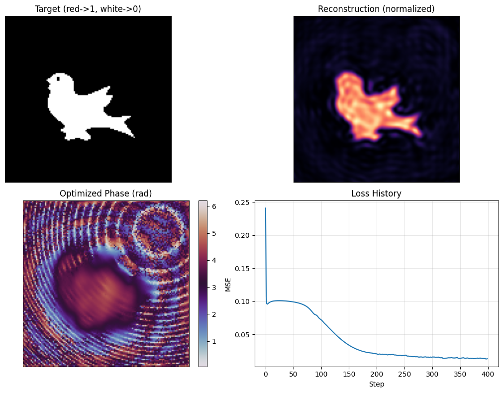
The final figure answers three practical questions at once: whether the logo is reconstructed, what phase pattern the optimizer found, and whether training converged smoothly.
A good result shows the normalized reconstruction concentrating energy on the logo region, while the loss history falls steadily. The phase plot is not expected to resemble the target directly; it is an interference pattern that only becomes meaningful after propagation.
if PLOT:
    fig, axes = plt.subplots(2, 2, figsize=(11, 8))
    axes[0, 0].imshow(np.asarray(target), cmap="gray", vmin=0.0, vmax=1.0)
    axes[0, 0].set_title("Target (red->1, white->0)")
    axes[0, 1].imshow(np.asarray(recon_norm), cmap="magma", vmin=0.0, vmax=1.0)
    axes[0, 1].set_title("Reconstruction (normalized)")
    phase_im = axes[1, 0].imshow(np.asarray(phase_opt), cmap="twilight")
    axes[1, 0].set_title("Optimized Phase (rad)")
    plt.colorbar(phase_im, ax=axes[1, 0], fraction=0.046, pad=0.04)
    axes[1, 1].plot(result.history)
    axes[1, 1].set_title("Loss History")
    axes[1, 1].set_xlabel("Step")
    axes[1, 1].set_ylabel("MSE")
    axes[1, 1].grid(alpha=0.3)
    for ax in (axes[0, 0], axes[0, 1], axes[1, 0]):
        ax.set_xticks([])
        ax.set_yticks([])
    fig.tight_layout()
    fig.savefig(PLOT_PATH, dpi=150)
    plt.show()
    print(f"saved: {PLOT_PATH}")
saved: /Users/liam/metasurface/fouriax/examples/artifacts/hologram_coherent_logo_overview.png